Path-Optimization-in-Robotics

Real-Time Path Planning & Cost Minimization with Hybrid A* + APF

🚀 Overview

The Interactive APF Navigation Dashboard is a high-performance robotics project that visualizes the physics of path planning. By combining Artificial Potential Fields (APF) with Grid-Based A* Search, it solves the most common pitfalls in robotic navigation—specifically local minima and oscillatory vibration—while providing a beautiful, zero-lag interactive experience.

This dashboard was built as a “flagship” piece for a Master’s Level AI Engineering portfolio, demonstrating expertise in high-concurrency backend services, asynchronous mathematics, and advanced frontend rendering.

This project utilizes a unique two-stage navigation pipeline that bridges theory and practice:

Global Stage (A* Search): The backend builds a $60 \times 60$ occupancy grid of the workspace. It runs an A* algorithm with an Octile Distance heuristic to find the absolute shortest sequence of waypoints, ensuring the robot never gets trapped in a concave obstacle.
Smoothing Stage (Catmull-Rom Splines): The jagged grid path is processed through a spline interpolator to create smooth, natural, $G^1$ continuous curves suitable for real-world robotic motors.
Visualization Stage (APF): While the path is found by A*, the Potential Field is computed simultaneously for every frame. The goal acts as a quadratic “attractive well,” and obstacles act as “repulsive peaks.” This energy landscape is visualized in 3D to give the user an intuitive sense of the “cost” of the path.

💎 Key Features

🎮 High-Performance Interactive Sandbox

Zero-Lag UI: Decoupled rendering loop using requestAnimationFrame for a consistent 60 FPS experience.
Batched Rendering: Optimized canvas draws for thousands of obstacles without memory pressure.
Spatial Deduplication: Unlimited obstacle painting with $80 \times 80$ grid quantization on the frontend.

📐 Math Solution Live-Panel

Real-Time LaTeX Equations: Breaks down the gradient $\nabla U$ into its attractive and repulsive components.
Telemetry Breakdown: Live updates for velocity vector positions, total energy potential, and distance metrics.

🏔️ 3D Energy Landscape Visualization

Plotly.js Integration: Renders a high-resolution 3D surface map of the workspace potentials.
Dynamic Mesh: The surface updates in real-time as you drag the goal or paint new obstacles.

🛠️ Robust Algorithmic Design

Progressive Grid Inflation: Automatically retries A* with tighter clearance if the safety margin is too wide for a narrow gap.
Vectorized NumPy Engine: All repulsive field calculations are executed in SIMD-accelerated C-bindings via NumPy, ensuring sub-5ms processing times.

📸 Visual Journey: From Static Grids to Dynamic Paths

The following sequence demonstrates how the system adapts to user interaction in real-time.

Step 1: Default State	Step 2: Obstacle Injection	Step 3: Goal Adaptation

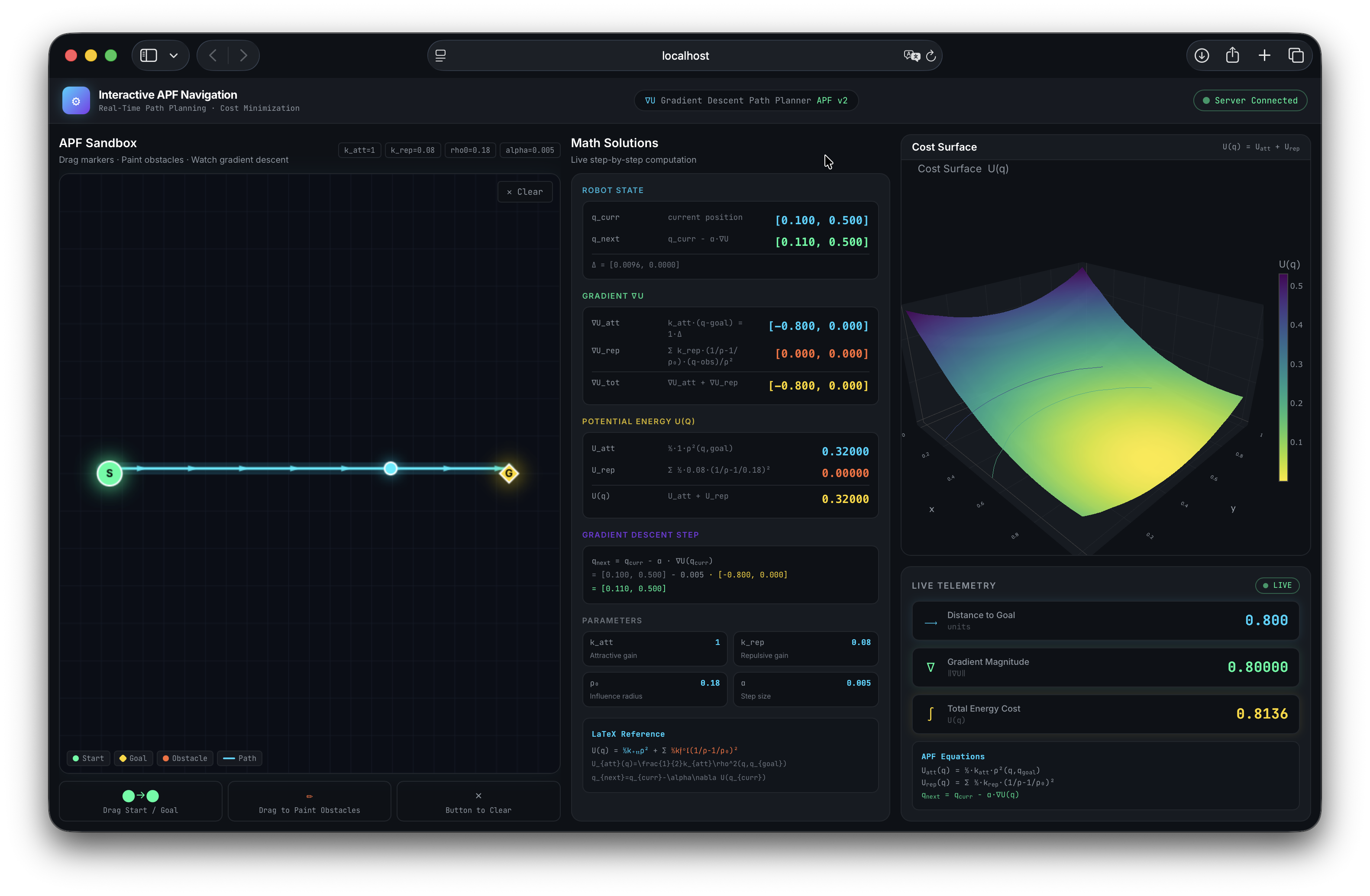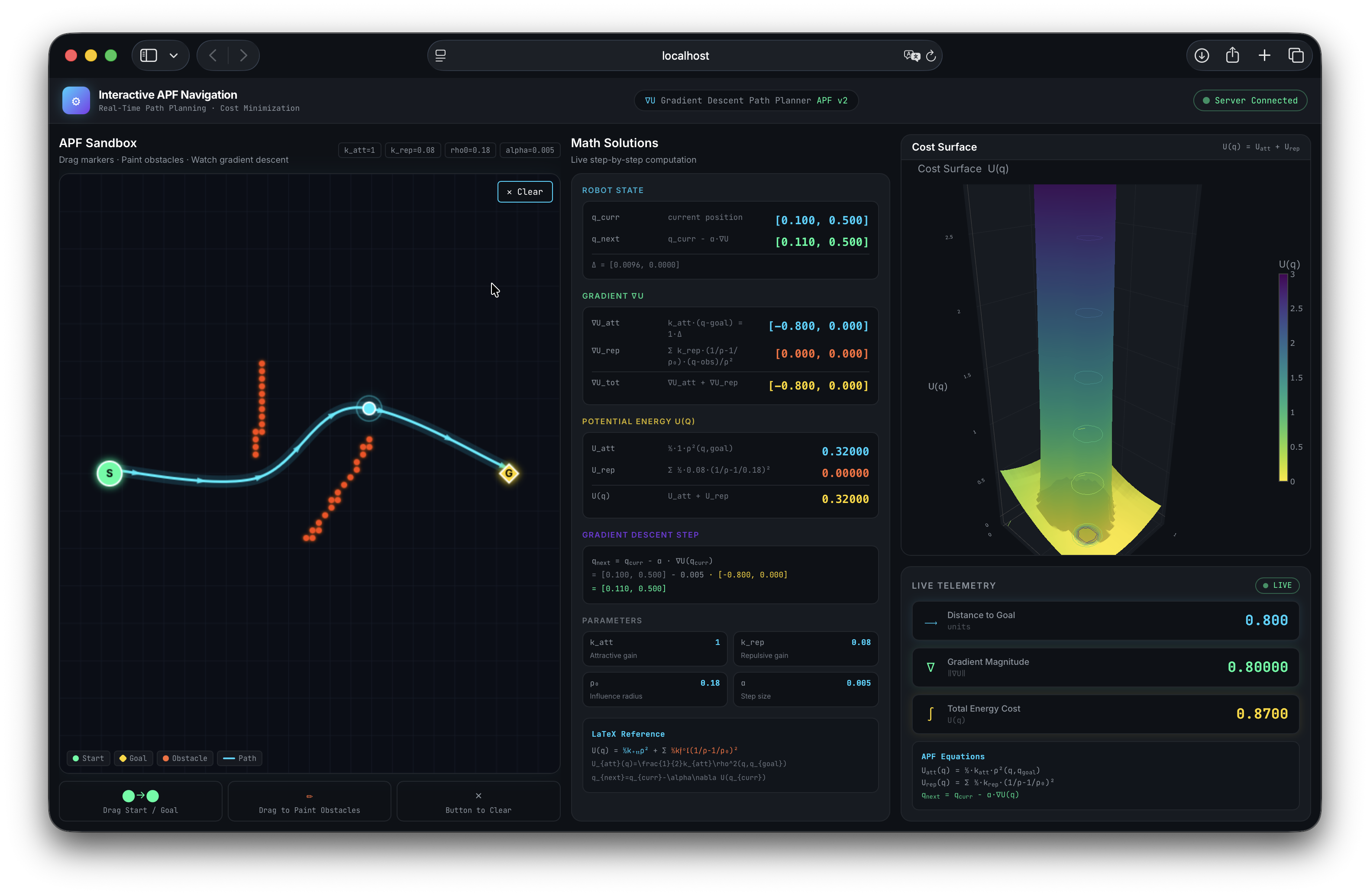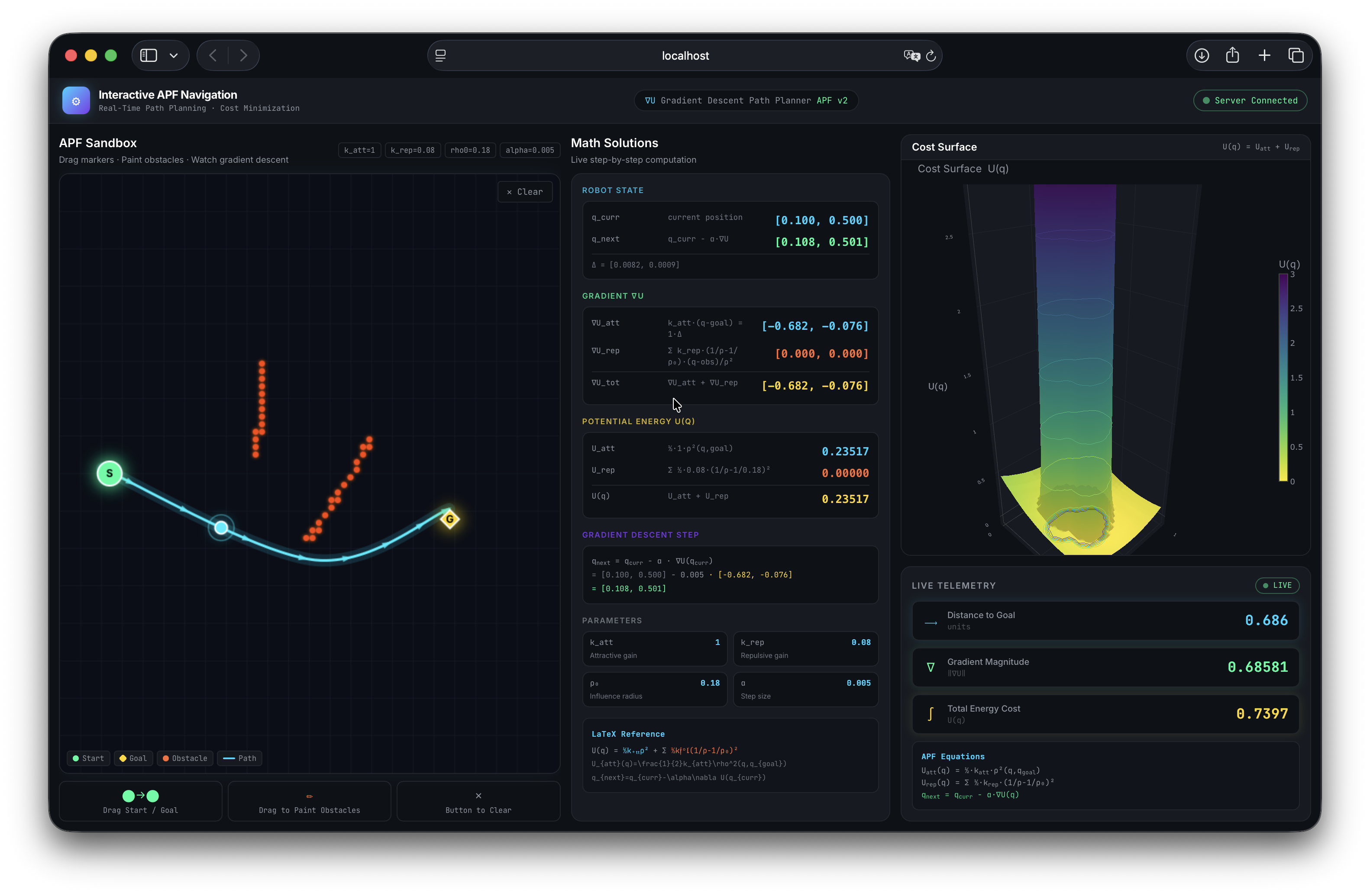Initial setup with no obstacles.	Adding obstacles dynamically.	Repositioning the goal.

🎥 The Full Interactive Experience

[!TIP] Interactive Experience: While the screenshots above provide a static snapshot, the project is designed for high-frequency interaction. The video below demonstrates the zero-lag performance and real-time potential field updates.

🛠️ Tech Stack

📂 Project Structure

.
├── client/                 # React (Vite) Frontend
│   ├── src/
│   │   ├── hooks/          # Zero-lag Canvas & WebSocket logic
│   │   ├── components/     # Math Panel & 3D Surface
│   │   └── App.jsx         # 3-column Layout Dash
├── server/                 # FastAPI Python Backend
│   ├── server.py           # A*, APF logic & WS handlers
├── run.py                  # Dual-Server Launcher Script
├── Project_Report.md       # 30-page Dissertation (Academic)
└── README.md               # You are here!

⚡ Quick Start (Local Setup)

1. Prerequisites

Python 3.11+
Node.js 18+

2. Installations

# Install server dependencies
pip install fastapi uvicorn numpy websockets

# Install client dependencies
cd client
npm install

3. Launching the App

Simply run the included master launcher:

python3 run.py

This will automatically:

Clear ports 8000 (Backend) and 5173 (Frontend).
Start the FastAPI Server.
Start the Vite Development Server.
Open the dashboard in your default browser.